Image Processing Techniques 2

When you open an image in CCDOPS, the software performs an automatic contrast adjustment.
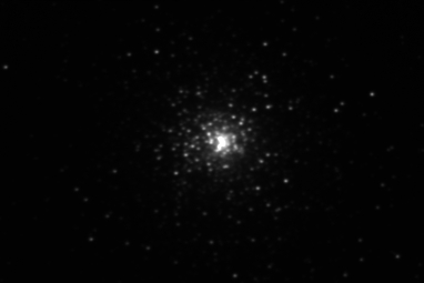
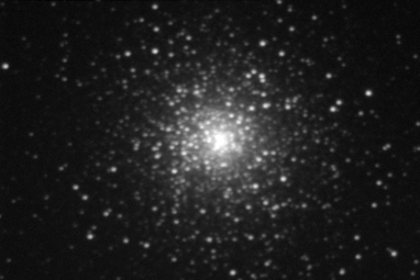
In most cases, automatic adjustment results in a globular that looks burned out (totally white), as shown in the example at left. In addition, many of the fainter stars are not visible. The core detail and the faint stars are there in the image, but you can't see them at this point.
You can usually get much better results by making your own manual contrast adjustments. In this example, the automatic adjustment resulted in a Back setting of zero, and a Range setting of 8764.
Back: The pixel value that will appear as black. All pixels with values less than or equal to this value will appear black in the image.
Range: The pixel value that will appear as white. All pixels with values greater than or equal to this value will appear white in the image.
Many of the pixels in the core have values greater than the default Range value, and that is why the entire core appears white. To show more of the core detail, you can increase the Range value. Click repeatedly on the up arrow just to the right of the Range setting.
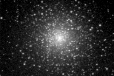
The image at left shows the result of increasing the Range value to show more core detail. The change in the appearance of the core isn't the only change, however. The stars around the core are now dimmer.
We have solved the problem of core detail, but we created a new problem to solve at the same time. We have lost even more of the faint stars in the image!
Before we solve the problem, let's look at why the fainter stars disappeared. That will provide some clues that will help us bring out the faint stars. They aren't gone; they are simply lost in the sea of data.
The diagram at left is called a histogram. It shows how many pixels there are in the image at various brightness levels. The far left of the histogram shows the darkest pixels, and the far right shows the brightest possible values. This particular histogram shows the spread of pixel values in the original image. Note that the pixels in the image actually occupy a very, very small portion of the possible values. This is typical in exposures of deep-sky objects. In this case, the data occupies a range from about 500 to less than 2,000.
The histogram curve looks suspiciously like a logarithmic curve, such as a parabola. However, right now the data is displayed in a linear fashion. That's not a good match for how our eyes actually react to light. To see all of the data in the CCD image, we need to adjust the histogram to display the data in a way that fits the eye's natural response.
The histogram also shows us that most of the data is scrunched into a small range within the larger range of all possible values. The CCDOPS Scale feature allows you to spread out the data to the full range by discarding the data that lays outside of a range that you specify. For example, a scale operation could take the values from 100 to 1,000 and scale them from 0 to 65,000.
The Utility | Scale... menu selection displays the dialog shown at left. It has three settings:
Background: This is the same as the Back setting in the Contrast window.
Range: This is the same as the Range setting in the Contrast window.
Log: This determines whether or not the operation will do log scaling when the image is scaled. "No" yield linear scaling, "Yes" yields logarithmic scaling, and "Auto-Log" will set the Background and Range values before performing logarithmic scaling.
The image at left shows the result of an "Auto-Log" scaling. Just about all of the core detail is visible, and most of the fainter stars have suddenly popped into view.
Compare this to the orginal image. The globular cluster is clearly much larger than you would have guessed from the original image.
No new data has been created in this operation. By scaling the data in a way that fits the way the eye sees things, more of the data already present can be shown visually.
The histogram at the left shows the result of the Auto-Log operation. The pixel values now occupy a much larger set of values, from about 31,000 to more than 40,000.
The curve of values is not as steep, and more closely matches the eye's natural response to light.
However, as with anything automatic, a careful human can often do better. The image at left shows a logarithmic scale where I set the values for Background and Range manually, based on my experience with this operation when adjusting images of globular clusters.
The next illustration shows the histogram for this image.
Notice that the pixel values are now spread out even more. The curve is even less steep than in the Auto-Log image, and the values range from about 12,000 to nearly 45,000. These values provide the optimal compromise in arranging the data for visual observation.
The core is now fully revealed, and fainter stars in the image are clearly seen. Images of many deep-sky objects, including galaxies, nebula, planetary nebula, etc. can benefit from a logarithmic scaling operation. The values will be different for every image, but using the concepts and guidelines from this article, you should be able to get results that will reveal otherwise hidden data in your images.